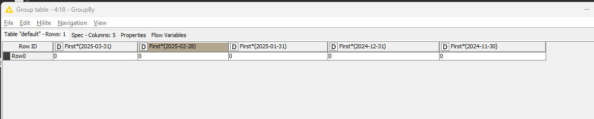
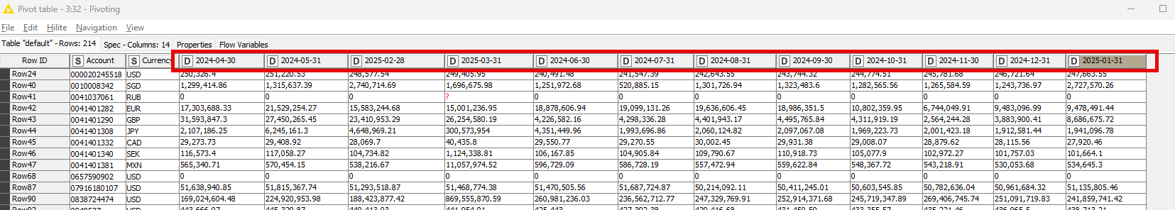
Here’s the final output I want: Final Output for 3months ( I only need the ‘Account’ and ‘Amount’ in raw data however need to change the Amount column name into its Last day of the month.
In short, every month it will be added a new data for the current month. So once I have added January, next month, I will add February then March so on until December then repeat to January again for new year.
Hope you can help me guys. Thank you so much as this is really hard for me to figure out.
Note: The account is being added or reduced every month though I still want to retain the old account and only add new account that will be added to preserve everything.
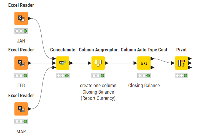
There is some inconsistency in your data. The data in the Closing Balance (Report Currency) columns are not always numbers …and have different names.
Closing Balance (Report Currency) #27
Closing Balance (Report Currency) #29
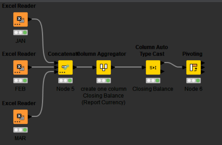
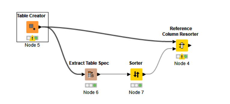
Therefore I added a Column Aggregator to be sure you end up with only one column containing Closing Balance information.
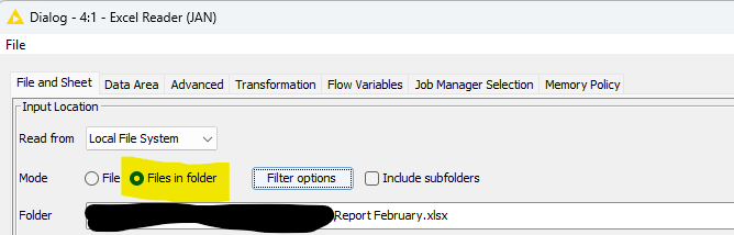
If you have all input files in the same folder than you can make use of the option in the Excel Reader, to read in all your monthly files at once. So you don’t need to modify flow (remove the Concatenate node, and connect the Excel Reader directly to the Column Aggregator)
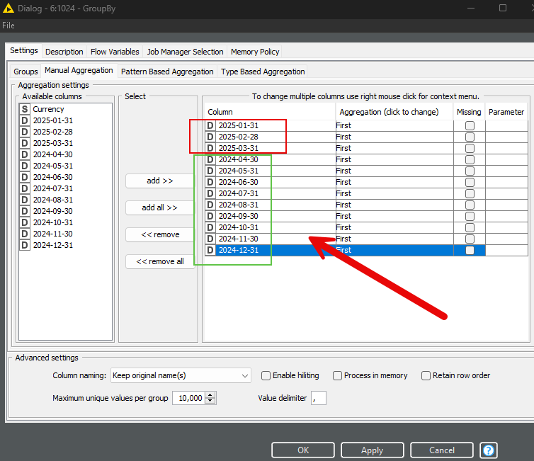
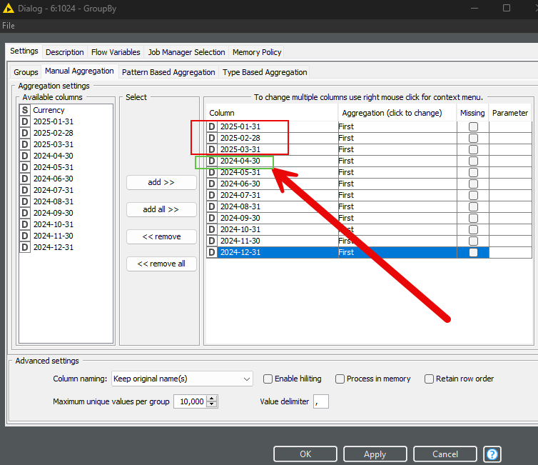
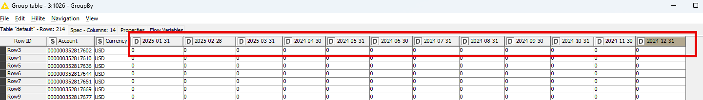
My question is, I am getting the right data already however, in GroupBy node - what if the 2024 data (highlighted in green box) will be replaced to a 2025 data for example the 2024-04-30 to 2025-04-30 hence it needs to be recaptured again or configured manually. It will also happen for 2025 when 2026 data kicks in.
Is there a way it will be automatic that data or columns in the manual aggregation will be added? Or Is there a another approach to do it? Thank you!
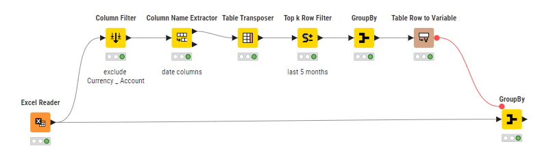
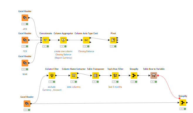
This wf select the 5 columns with the most recent dates. So when your excel is updated with a new column name (recent date), the GroupBy is performed with those new set of column names.
Hello @HansS - sorry for the confusion. What I meant was, For all these columns in Groupby that I’ve set is all good with the data I have. However, if I will have a new data, the 2024-04-30 will be replaced as 2025-04-30 hence the Groupby node will not read the 2025-04-30 in this manual aggregation because it is a new column.
So my question is, how can I ensure even that I have new data with new months, it will still be captured.
you can use the “Pattern Based Aggregation” tab or “Type Based Aggregation” tab.
In the first you can define a pattern to select all columns like “--*”
In the latter one you can select the “double type” columns.