I’m sure I’m doing something wrong. I got excited after attending the Time Series Training at Summit.
I get 0.0 for both Seasonal Component 1 and 2…
I imported the data then applied the Timestamp Alignment component and then used Missing Values to fill in gaps and finally connect to the Decompose Signal. The file below is the table just before the Decompose Signal.
Shouldn’t I get something even if very small? It feels like it’s just not calculating.
Looks like I just don’t have enough data. My data is Daily sales data from a cafe. If I want to see if there is any seasonality… i.e. over a week or across months… how much data do I need? I have 520+ days of data. What should I be setting the Max Lags and Lag Steps and Correlation Cut-off at? I had tried Max Lag =7 and Lag Steps = 1
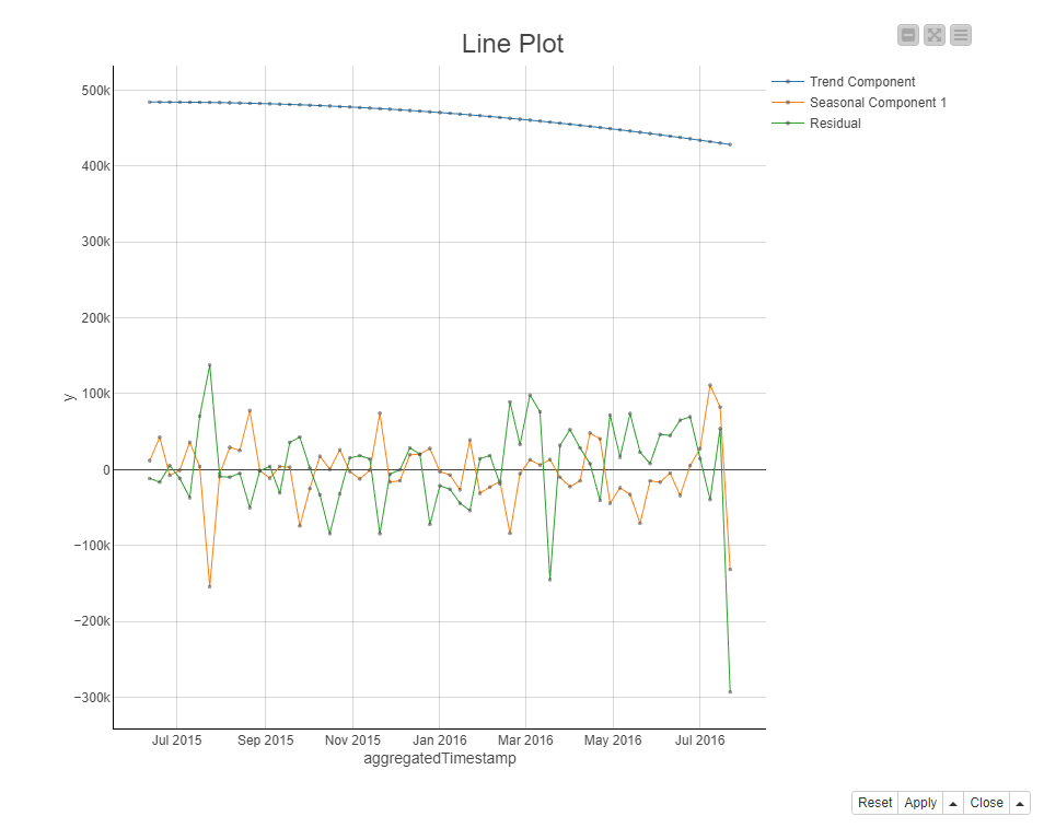
And this is the output I expected to get (trend and seasonality components) for each StoreID:
I thought I could just use a Group Loop Start (StoreID) and use a component to calculate the Trend and Seasonality… But the Decompose Signal seems to generate this for each row (which was a surprise) as I’m looking for metrics for the entire data set by StoreID. Maybe I’m using these components incorrectly.
Hoping someone can show me the light as I have been wrestling with this all day.
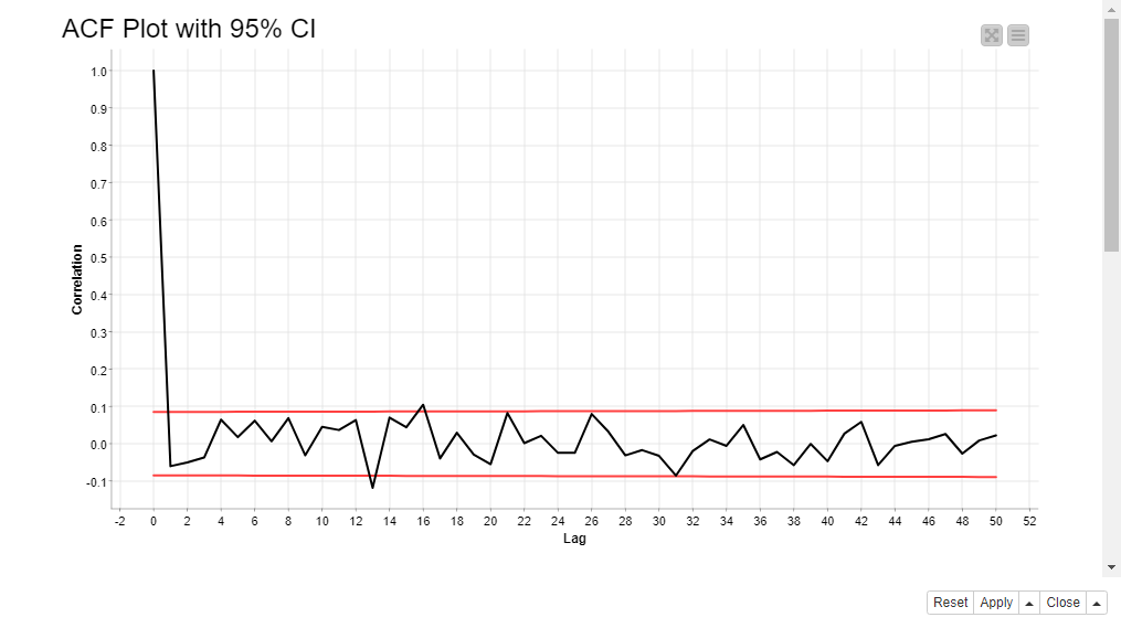
Hi, I checked your data, and as you can see from the ACF plot below, there is no significant correlation between the current value and any lagged value, and that’s why the seasonal components given by the Decompose Signal component are 0.
A rule of thumb for how much data you need is 4 seasonal cycles. Therefore, if you want to inspect weekly seasonality in daily data, you’ll need ~47=28 data points. If you want to inspect yearly seasonality, you’ll need ~4365 data points. However, often already fewer data and domain knowledge give you an idea what kind of seasonal patterns you might find in your data.
If you want to inspect weekly seasonality with the Devompose Signal or Inspect Seasonality components, the max lag value should be at least 7, but it’s good to set it at 30 or more to see that the max lag value repeats at lags 7, 14, 21, 28, and so on. If you want to inspect yearly seasonality in daily data, you’d need to set the max lags at 365 or more.
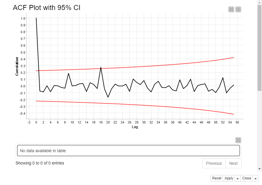
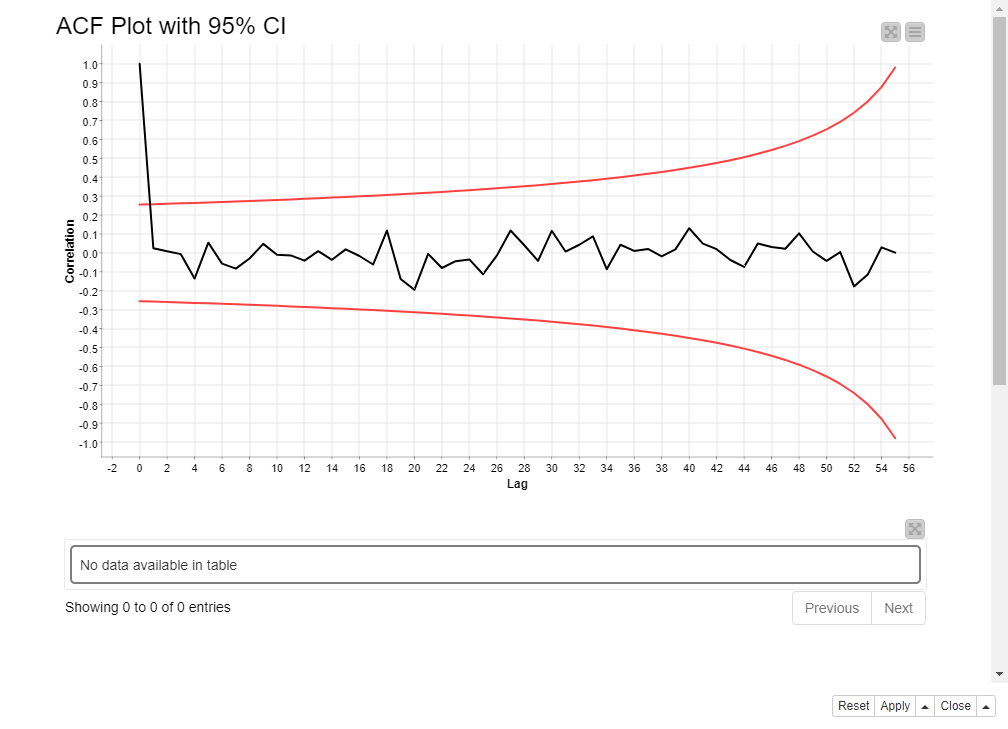
If you wan’t to model the weak seasonality at lag 18, you can do it by lowering the cutoff value from 0.5 to 0.2. After differencing the data at lag 18, the ACF plot looks like this:
If you’re wondering why the trend component is shown for each row, the Decompose signal calculates a regression model for the trend component and the value in each row is the output of the regression model for each row index. If you sum up the values in the residual, trend, and seasonality columns, you’ll get the original value of the signal.
Thank you so much for the detailed explanation… I’ve been learning a lot from you in the last 2 weeks.
If I want to understand the trend for all of the points do I just take the mean? of the trend for all the points? Not sure if statistically makes sense. What I’m trying to do is have a way to compare stores and include trend and seasonality as components to understand how similar stores are to each other.
So I will want an overall trend and overall seasonality.
Also I’m not sure if I need to do any processing on the trend to make it comparable across stores. maybe turn it into a percent by dividing the trend by the total gross margin?
I’m an amateur… open to suggestions. Do you have thoughts on a better way to compare sales data of stores?
If you want to compare the trends of two time series, you could plot their trend lines in a line plot. This way you can say if the trend line has the same shape for both time series, and if it’s increasing faster or slower for one of them. The same is true for seasonality - you can inspect the lengths and magnitudes of seasonal cycles in a line plot and compare two time series. The figure below shows your time series decomposed into a trend, seasonality, and residual, as produced by the Decompose Signal component:
If you want to calculate statistics for the time series, it’s recommended to do it separately for each season. For example, if you have weekly seasonality, then calculate statistics for each weekday.
The error in the component might be because the max lag is equal or greater to the number of rows in the input data. If your data has 77 rows, try for example max lag=50. Do you still get the error?
You are right. when I reduce the lad to 50 I can set the correlation Cut-Off to lower. I don’t recall if we covered in the L4-TS training how the Correlation Cut-off is affected by the number of rows of data. I think I might have to rewatch the video and look at the slides again.