Hi @Ashwath5245 ,
I’ll try to do a quick “Continental Nodes for Dummies” (or Continental Tutorial-Lite), as the main Continental FAQ Page is the primary source of info for links and the more detailed description, and to be honest, it took me a while (and a fair bit of reading of posts such as to get to grips with them.
The trouble is that the XLS Formatting nodes are actually really simple but kind of complicated at the same time. The concept is straightforward and yet seems complex…
So where to begin…
In simple terms you have the following concepts. Don’t worry for the moment if my brief definitions don’t fully explain them. I’ll try to expand on them in a moment:
-
Your Data
You know what this is, and basically its your data that is going to get written to Excel -
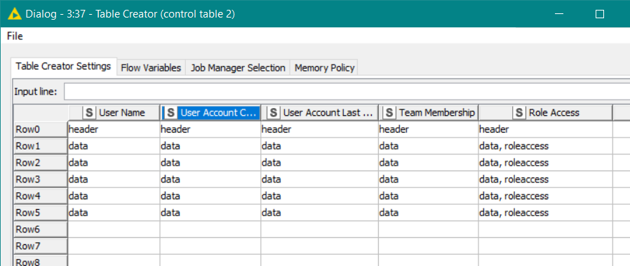
Control Table
This is a table of information containing a row and column for each row and column that appears in your data, plus an additional row at the top that contains information about your Table Headings (column names). Each cell of this table contains “tags” -
Tags
This is just a set of “labels” that you create and assign to one or more cells in your Control Table, to be used by the formatting nodes.
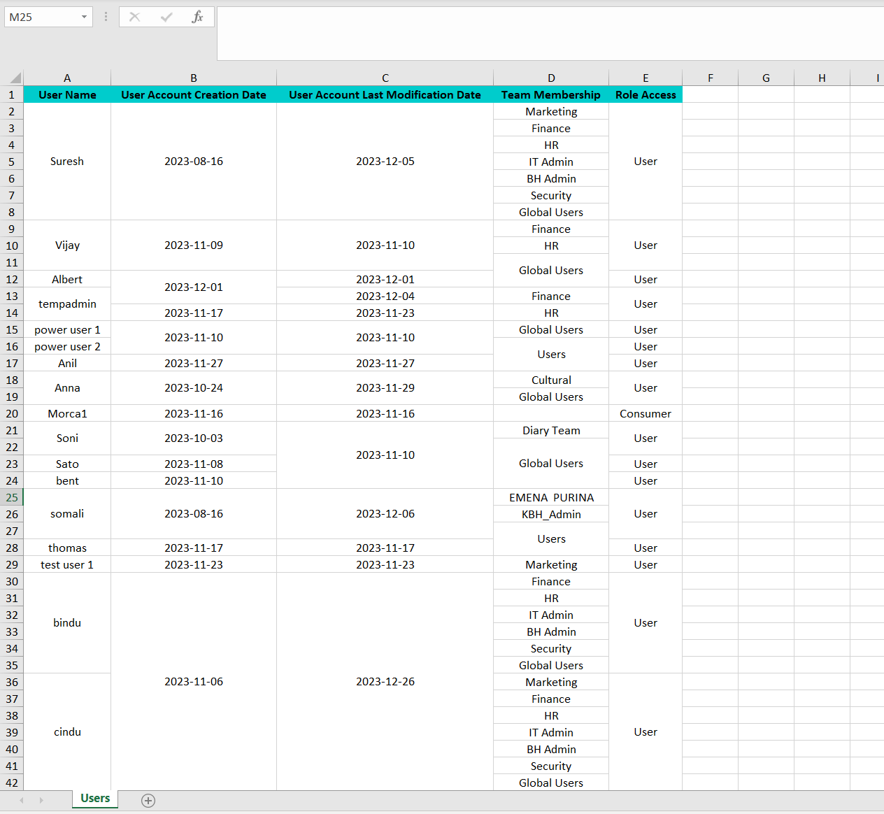
Right, let’s use a small sample of to give some background on how this works. I’m just going to start by showing how you can format the first row to be black text on a light blue (cyan) background
Your Data
I’ve taken a subset of your data for demo purposes, and put it in a Table Creator node
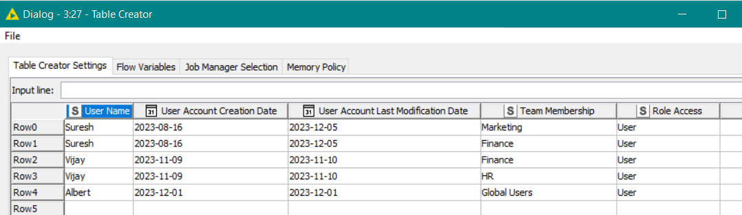
What we want to do is to output this to Excel with the first row being formatted as described above (light blue background with black test).
The first step is to decide which cells in the output xlsx will have formatting applied. That’s fairly easy in this case as it will be the “header row”. Of course in your data table, there is no “header row” as such as the table has dedicated “column headings”, but when it is written to Excel, the first row will be the “header row” which will contain those headings.
Control Table and Tags
To build the Control Table, we “simply” make a table defining all the cell positions in the resultant XLSX where the first row is all “header” rows and the lower rows are all “data” rows. We could start by defining this:
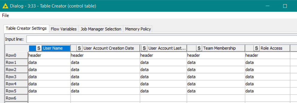
Note that the columns are all “String” datatype as we are placing text strings in each position. The first row of cells say that it is a “header”, and the other rows all have the word “data” in them. I could use any words I wish. They could simply be H and D or they could be Title and Body. It doesn’t matter what “labels” you use. Anyway these labels are what Continental nodes refer to as “tags”, and the above image is the source for making a basic “XLS Control Table” for the continental nodes.
To turn that into an actual control table, we need to rename the columns as A… E and the rowid needs to be come a sequence of numerics beginning at 1. We could do that manually with a few nodes but the Continental Nodes provide us with the XLS Control Table Generator to do exactly that
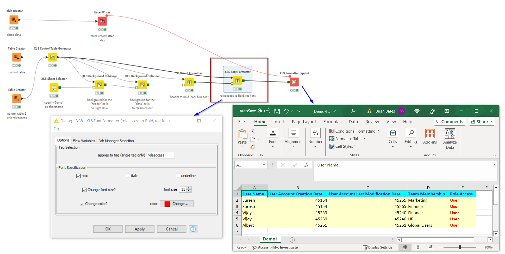
This is what my workflow looks like so far:
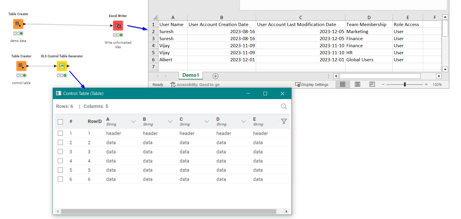
It’s not very fancy yet, and the output is still quite boring, but you can see how the “tags” in the rows of the control table align with the rows and columns in the Excel output.
Clearly we need to do something with that Control Table which is sitting idle, so that it changes the format.
This is where we start using the Continental XLS formatting nodes.
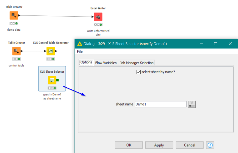
The first thing we probably want to do is tell it the name of the sheet. You can see in the above screenshot that I’m calling my sheet “Demo1”, so I’ll add an XLS Sheet Selector node, and configure it:
After that we start doing the fun part ![]()
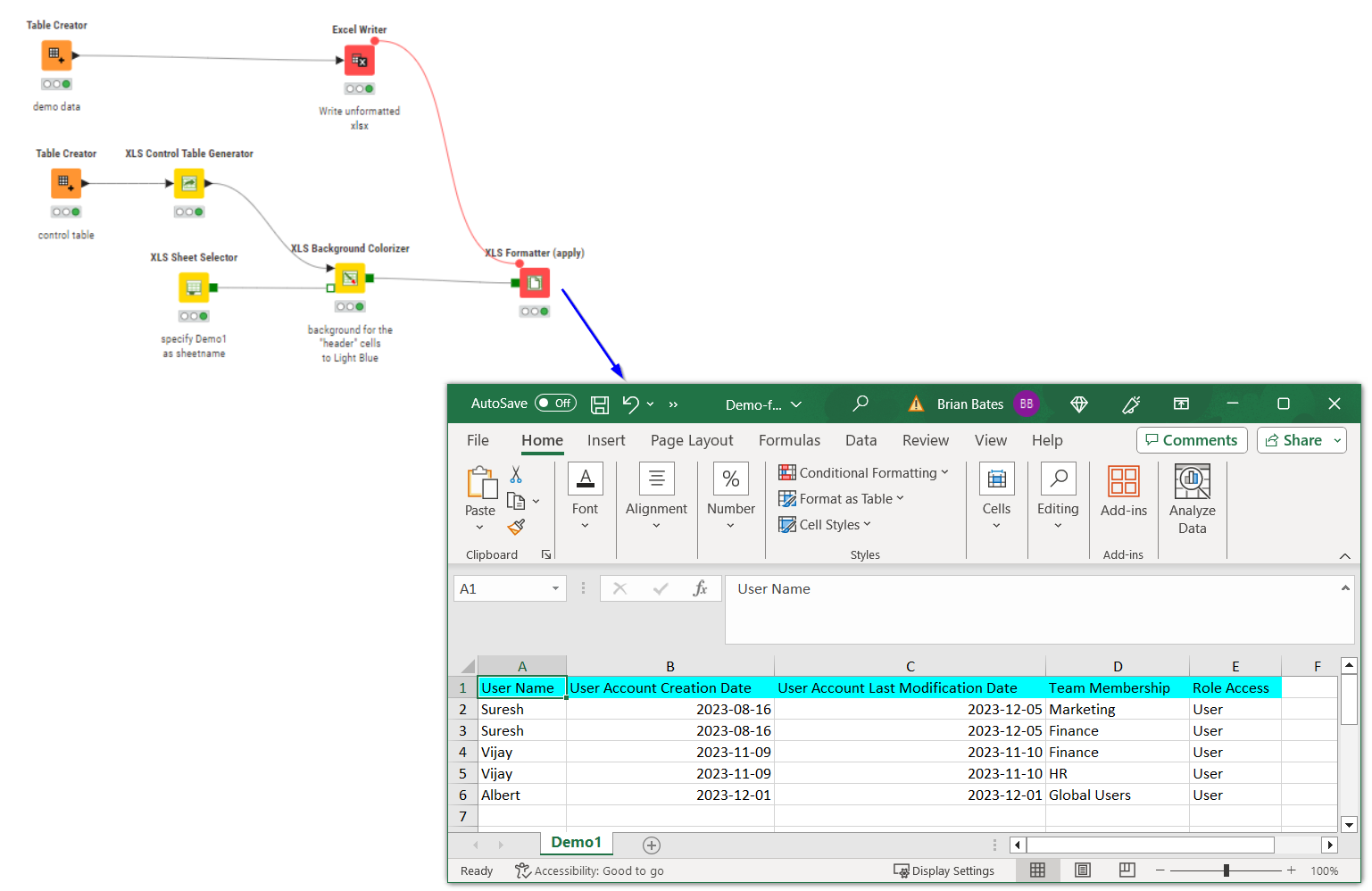
Let’s set the background colour of any cell containing the tag (label) “header” in the Control Table. We do this by adding an XLS Background Colourizer, and setting the background colour to the cyan colour. We tell it the name of the tag to which this colouring should be applied, by writing the word “header” in the Tag Selection box.
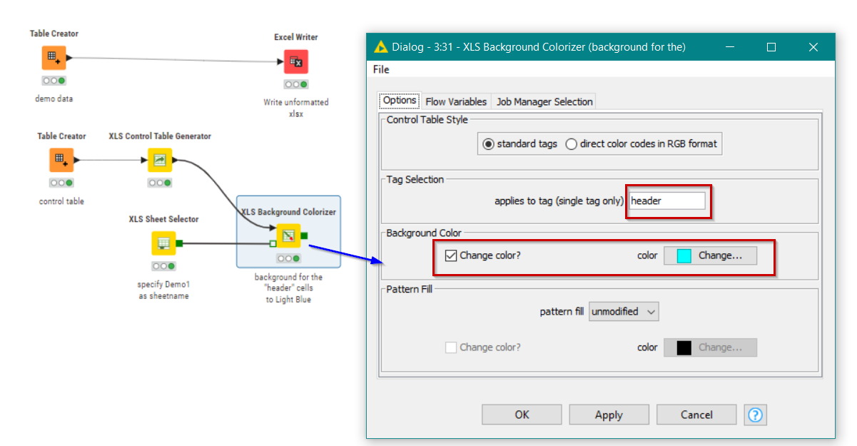
Since every cell in row 1 of the Control Table contains “header”, when this gets applied to the spreadsheet, the column headings in row 1 will all be set to light blue background.
But to do that, we need to somehow apply this formatting to the spreadsheet, and this is where the “finalisation” node called “XLS Formatter (apply)”
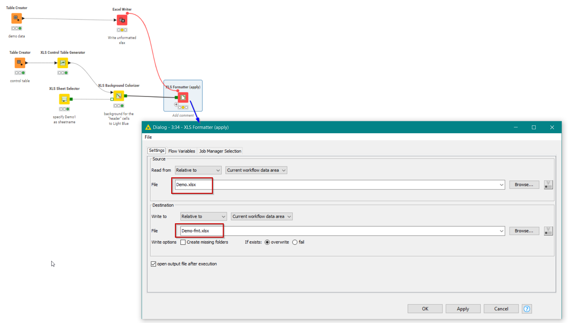
You can see that this is configured to read an XLSX file that has been generated with the data, but without the formatting, and then it writes a new XLSX file which is formatted using the information from the Continental XLS Formatting nodes. Also note that a flow variable link is added in my flow between the Excel Writer and the XLS Formatter (apply) node. In this case it is there purely to ensure that the non-formatted xlsx already exists before the attempt is made to apply formatting.
And that is essentially it as a kind of “Hello World” tutorial on formatting a spreadsheet with the Continental nodes.
Adding more formatting is generally a case of adding further nodes in sequence, each feeding to the next, and each receiving the same Control Table, so we can change the background colour of the data rows, and the text colour of the header rows:
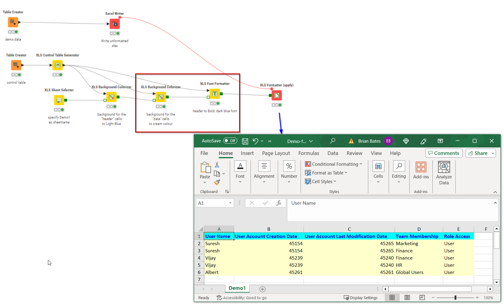
One other thing I should have mentioned with the Control Table is that a single cell can be allocated more than one tag, so that it can receive various formatting instructions depending on its position.
Supposing for example, you wanted the Role Access data to be red… Then you might have a Control Table that looked like this:
and you could add additional formatting for the “roleaccess” tag which would output the xlsx like this:
Now, I found that in general, the biggest hurdle to working with the Continental nodes came in understanding (and building) the Control Table. As you can see the control table is relatively simple in basic form. But building it can take a little time, and building it dynamically so that it varies with your data is somewhat more of a challenge than just building a static one like I did in the above example.
The static example shows you what you are aiming for but then to do that with a varying number of columns and rows is where the “simple” becomes “complicated”.
And when I was faced with that part of working with these nodes, I decided that I was going to need to find a way of making “complicated” back into “simple”, or… at least less complicated!
Which is how it is that writing this is the first time in a while that I’ve gone back to basics to explain how these nodes work, and why… I never do it that way! ![]()
Because I wrote a bunch of components to take away the pain and mean I no longer had to really remember how it all worked (until today!).
The first of these components, is the XLS Control Table Auto Tag Generator. A bit of a mouthful but it does what it says on the tin. It automatically generates a whole set of tags in a Control Table based on your data. It essentially builds the tags that I am most commonly going to need, and also allows you to specify the sheet name, so you can do without the XLS Sheet Selector node too.
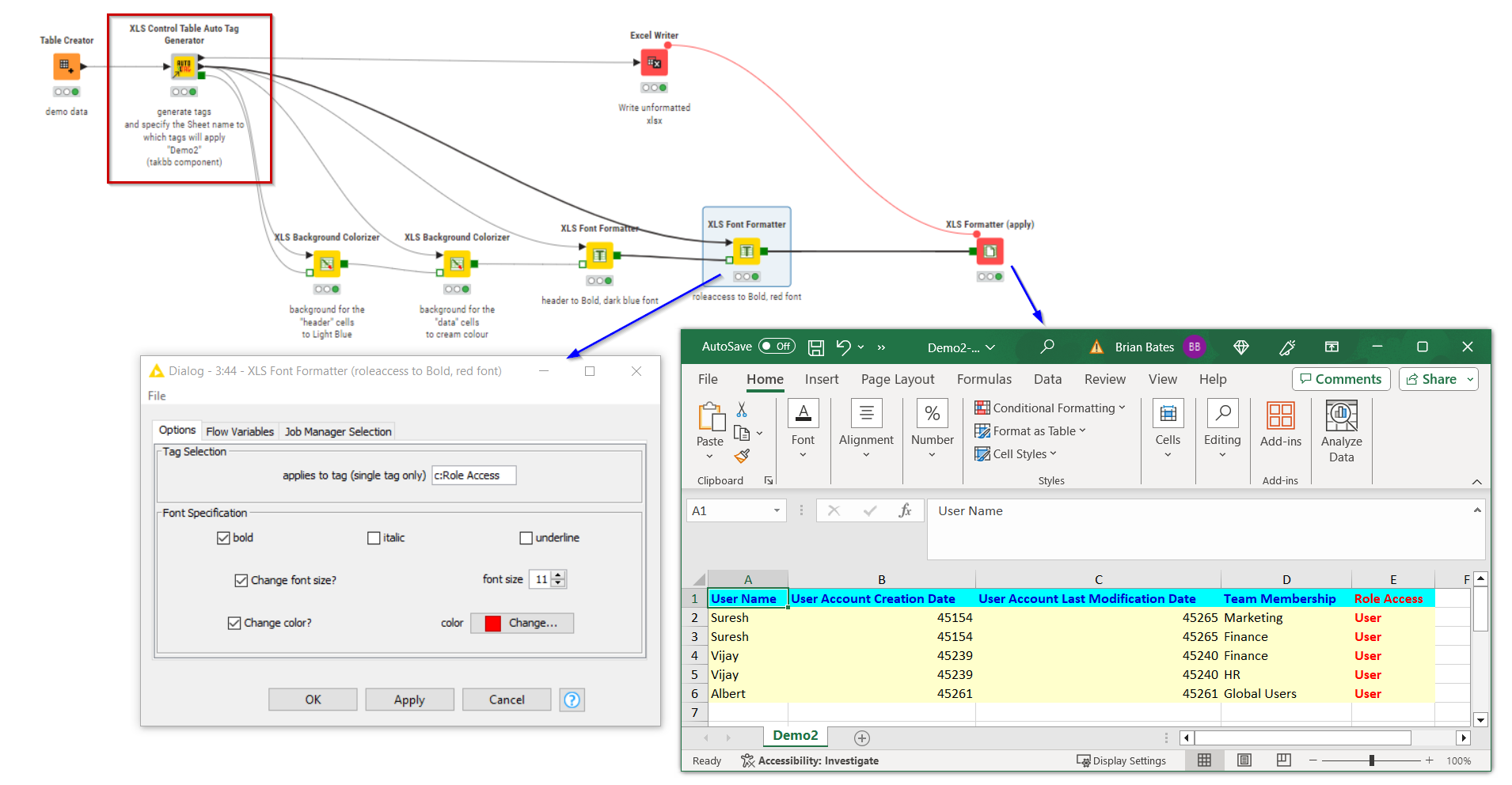
Notice that the highlighting of the Role Access column data in red was still achievable just using the auto generated tags. This is because for every column it automatically generates tags for that specific column name.
h:Column Name (identifies the cell that is the header for the column)
d:Column Name (identifies all cells that are the data for the column)
c:Column Name (identifies all cells for the column)
Here is the generated control table for the above data:
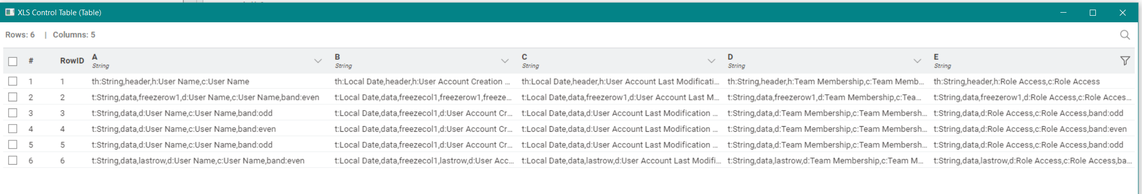
Along with that, as you can see you automatically get tags identifying the header rows, the data rows, a t:tag which identifies data type, so you can format all t:Local Date columns a particular way, for example.
The data cells in the final row are identified by lastrow tag, and you can also freeze row 1, along with a number of columns (specified in the config for Auto Tag Generator) by using the XLS Sheet Properties tag, telling it to freeze panes at the freezepanes tag.
So I hope that has given you a useful introduction to how the Continental nodes work, but also given you an idea of how to perform simple formatting by making use of my Auto Tag Generator component. You don’t have to use it, and there may still be times you need additional tags, but for general formatting of headers, data and data types, it provides me (and hopefully you) with what is needed.
So now… back to this thread and your need to merge and format cells. Using all of the information provided in this thread so far, with the components for performing merging, and this new post that demonstrates formatting, we can do the following:
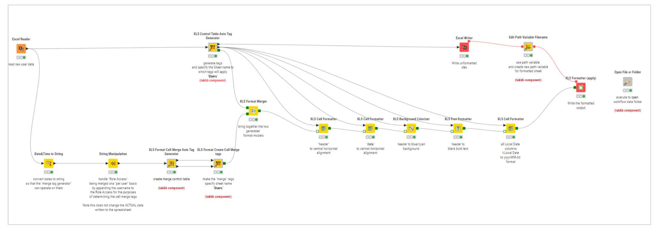
The upper branch uses the Auto Tag Generator and you can see that it performs the cell formatting that I’ve just been describing, along with additional formatting for cell horizontal alignment, and formatting of dates.
The lower branch performs the creation of the cell merging tags as described before. I’ve made a couple of modifications to those components for improved performance. Merge tag generation takes a little longer than I would like, and there may be further improvements in future but for the moment it does the job.
You can see that the output “models” (the green square ports) from the upper and lower branches are merged together using the Continental XLS Format Merger, which is useful to know about if you need to add further tags to those generated by the Auto Tag Generator.
Beyond that, hopefully it’s self-explanatory. This is what it produces:
This is the workflow using KNIME AP 5.2
Formatting Excel 1.knwf (677.0 KB)
It turned out to be not quite so quick ![]()
Anyway, you may wish to also read my post from Sep 2022…