Hi, you could do it something like this. I created two additional columns using Rule Engines.
The first determined that if a Quote wasn’t present, we could treat it as 1, because we were going to multiply it, so I built a column that was either the stated Quote, or 1. I could have replaced the Quote column but decided to not replace your data.
The second rule engine did a similar thing for Average Price. It created another new column which chose either Average Price, or Alt Average Price if the value of Average Price is 0.
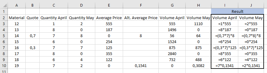
So after that the Math Formula can be used for April and then for May simply by multiplying the two new columns by the required Quantity UseQuote * UseAveragePrice * QuantityApril.
It is possible to put if conditions into the Math Formula node, but in this case I determined it was easier/cleaner to use additional columns. I added some rounding in the Math Formula node that you or may not need.
I did get slightly confused because your spreadsheet’s values for Volume April and Volume May don’t always match your required result.
As your spreadsheet already contained Volume April and Volume May, I didn’t overwrite them (although I could have done that in the Math Formula nodes). Instead I created two additional “result” columns. Lastly I filtered out the working columns from the result set. KNIME_excel_math_formula.knwf (23.0 KB)
Hope that helps
Indeed, line 5 seems to be a mistake for the results from @ARock1980 . I’ve not downloaded @takbb 's workflow, but from what you wrote @takbb , I am guessing your 2 new columns are for for:
Quotes:
Missing Quote or Quote = 0 => 1
TRUE => Quote
as UseQuote
Average Prices:
Missing Average Price or Average Price = 0 => Alt.Average Price
TRUE => Average Price
as UseAveragePrice
And like you said, just multiply the Quantity by these 2 new columns.
Yes actually I should have included the OR statements you mentioned as for the “Missing” values, I used Missing for one and 0 for the other, based on the Excel. So your conditions would be better and safer!
I was additionally trying to think of a way to not have to put in a node for each month. So far I’ve come up blank.
I couldn’t find a way of doing it with multi-column as I don’t know of a way to reference “Quantity April” from “Volume April” and then “Quantity May” from “Volume May”. You wouldn’t want to keep adding nodes when June, July etc come along
Ideally I’d put it in a column loop for all the “Volume*” columns, but referencing a column by variable name in java snippets, or maths formula etc doesn’t seem possible in the places I’ve looked so far.
Possibly transposing/pivoting the columns into rows briefly could yield the value… ?
@mehrdad_bgh, your use of the Column Expressions node was the answer I needed to find a way of making “variable column names”, so we don’t have to write code specific for each month.
I got it to work, in that it finds all the “Quantity [monthname]” columns and for each one works out a result column.
The thing I haven’t figured out is why, after I’ve looped the columns, it doesn’t put the columns in the same order it found them… !
You always have more flexibility with Column Expressions because you can “write code” if a manner of speaking, but I thought you guys wanted to stay with the Math Formula node
@takbb , regarding the order of the columns, it is actually putting them in the same order it found them, but it is not what you expected to see
To understand this, you have to run the loop 1 iteration at a time - well, at least the first iteration to understand what is going on.
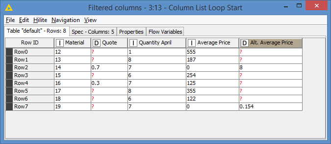
This is from the first iteration:
So, essentially before it starts the loop it has all the columns except for the Quantity columns, and at first iteration, it adds the Quantity April wherever it was found and processes whatever it’s processing within the loop.
In the next iteration, it will be again the same columns but instead of Quantity April, it will do Quantity May. What you have to realize is that it will again have 6 (5 input columns + Result column) columns, which it will try to append after the 6 columns from the first iteration, so now you have 12 columns.
And so on until the loop is done. That is why you end up with 30 columns at the end of the loop (Node 23), in that same order of the 6 columns repeated. And of course, the column filter only filters out the columns that you want to remove, keeping the order as is, and that’s how you end with the 6 columns from the first iteration, and then a pair of Quantity and Result after that.
Thanks for that explanation @bruno29a, I can see what you are saying, and yes that makes sense now.
So my next thought, is I wonder how to programmatically rearrange them at the end so that they then follow the order of the columns on the original excel and then have the result columns on the end - maybe join back on the original sheet in row order and discard one set of matching columns maybe? Is there a better method?
Regarding maths formula or column expressions… Yes my original thinking was trying to do the “no code” rather than “code” route. But I’ve only headed down this path so I could get variable column names to work. Being a programmer, I really don’t like a hard coded solution (or one that’s not future proof) if it can be avoided
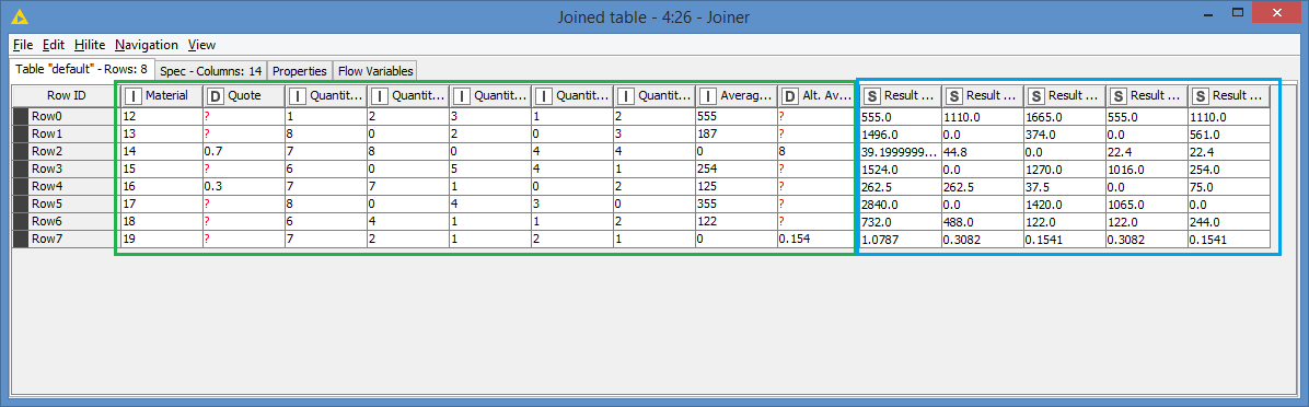
Hi @takbb , the only way I can think of to keep the columns in the same order as the Excel file without having to manually select the columns is to have the Excel table as left table and join with the results.
I gave it a go and it worked, but not sure if it’s the optimal solution.
As you can see, the original columns from the Excel file are in the green box and the generated Result columns are appended after in original columns, in the blue box.


 )!
)!