So I’m running a linear regression analysis to look for variables that can explain the variance of salaries. I’m running different types and different combination of variables that are all text. For example, are you a manager vs not a manager, your gender, Are you in a major city or not, what level are you and so on.
To my question - in the output of “Coefficient and Stats” they list each value within that variable that I’m testing against and list the (Coeff, Std error, t- value, P - value). My issue is for whatever reason certain values (just one) within a variable (my X) are not listed in this table?
For example, when I test the gender variable it has both women and men, but only the variable Male is listed in the table providing the metrics that I listed above (i.e Coeff, so on). Why does this happen? is it stating that Females are the intercept? and that is why it isn’t listed?
This also seems to be a trend with each of my variables to where it is missing one value from the variable (my X). Another example, where I have your level in the org which can be ten values. The highest or lowest one is missing. Once again, does that mean that value represents the intercept and that is why it isn’t listed?
Your “text” variables should be coded to dummy or ‘indicator’ variables (i.e. 1 or 0). For example if in your data set you have Male or Female, and Male is categorized as 0, and Female as 1, then the coefficient for gender is only related to female, as coefficient * 0 (male) = 0. The same is true for your other categorical variables. You should always have N - 1 the number of categorical variables coded as dummy variables. That is to say, if you have 10 levels, you would have 9 columns representing the 10 levels with a 1 in row that corresponds to the level of the person, and 0s in the remaining column. If all columns have a 0, then that means the person is level 10.
Hope this helps. This seems more like a stats question than a KNIME question.
Sorry that it isn’t Knime related and stat related, but I have one more question that I would greatly appreciate if you could help wrap my head around it.
So it is similar to my first question but one step further with a question of the quality of my multi-linear regression model.
I have noticed that R Square values can vary dramatically depending on how I step-up my X variables in Knime (I know it is still more stat related) and wanted to know your opinion is one method better or worst than the other.
So to put out a simple example, so my Y variable is salaries and my X is level in the organization and want to use this regression model to see if my levels can predict salaries.
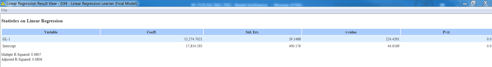
in one case, if I setup my levels as numeric value in the linear regression node it will show up as one variable and give me the R2 of (68%), and let me know the coefficient increase as each level increases.
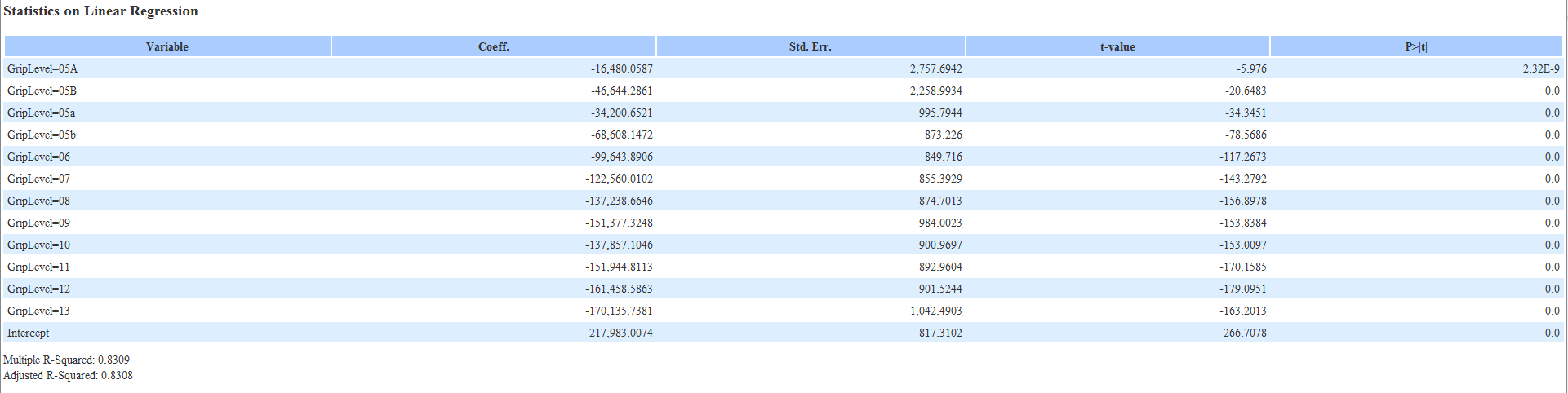
Now, using those same levels as text. I noticed that knime sets up each level as a individual variable (as 0 and 1) (1 if they happen to have that level and 0 if it doesn’t). Here, I will has many variables as levels I have instead of one. The interesting thing here is using this method my R squared goes up to 83%.
Finally my questions, based on the results it would seem it would be better to use the second method. Therefore, is there any pro/cons setting up a regression model this way?
Hi @guard88,
Interesting question. I think part of the answer lies in understand the interpretation of the two models. In the first model, it would be interpreted as: “Base salary of $17,854 and for every additional increase in level, salary increases by $13,274”. In this instance, there is no “cap” for number of levels. So you could project the salary of a level 50 employee, if they were to exist. (In this case… $17,854 + $13,274*50 = $681,554 == projected salary for level 50 employee)
In the second model, you don’t have unlimited runway. Your model is interpreted as, “The starting salary is $217,983, and if you are level X then subtract $Z from the starting salary.” The difference here of course is there are only certain number of levels you can subtract from the starting salary. You cannot project what a level 50 employee would make in this model.
Therefore, I would tentatively say that the second model is more accurate… However, accepting or rejecting a regression model solely based on it’s R^2 value is a dangerous thing to do. You should do residual analysis, and check for things like heteroskedasticity, etc. It is possible that the second model, while having a higher R^2, may violate some of the assumptions of linear regression, and therefore the first model may be better.
Thank you for telling me to look into doing a residual analysis to check for heteroskedasticity and I will surely do that. I have been researching online of different method on how to do that and I was curious does any of the nodes in Knime to help with this analysis or no? This is only from one hour of research, but I was seeing to do things like spitting your population in half and testing for P values (I know I’m most likely over simplifying it).
Now to your comments on the two models that I shared above, to give you additional context. I’m doing an analysis for a organization by using linear regression to identify variables that help explain why we pay the way we do (i.e Level, Location of person, type of role, manager/non-manager, Tenure, and so on). From there, the idea is to use this model to predict the employees salary based on the model and see how much it differs from their actual salary. The ideas is to use this analysis to look for any potential bias in pay towards a protected group. Based on this, I have a clearly defined set of levels in my organization along with my other variables. From what you explained above my dataset would never have levels outside the 13 levels that I have in model 2, so having the unlimited runway in model 1 would actual add no additional value to me. Therefore, I would assume in the context of this simple example model that model 2 would be the preferred model (of course I need to additional validation to truly confirm that).
No, KNIME doesn’t have a specific node that does residual analysis that I know of, but it can be calculated done very easily. I’m doing this from memory, so hopefully my steps are correct:
Residuals are calculated as (Predicted Value - Actual Value)
After creating the model with the Linear Regression Learner node, run the model through the Regression Predictor Node (This will append a predicted value to the table)
Use the Math Formula node to subtract the Predicted value from the Actual value to create a new column called “Residual”
Attach either a scatter plot node or a histogram node to the result. If you view as a scatter plot, the residuals should be spread evenly. If you look at the residuals via a histogram, the histogram should follow a standard normal distribution (bell curve)