Tune a Simple Keras Feed-Forward Neural Network

[Edlueze]

Can somebody please help me tune this neural network?

Simple Demand Forecast Neural Network 001.knwf (3.4 MB)

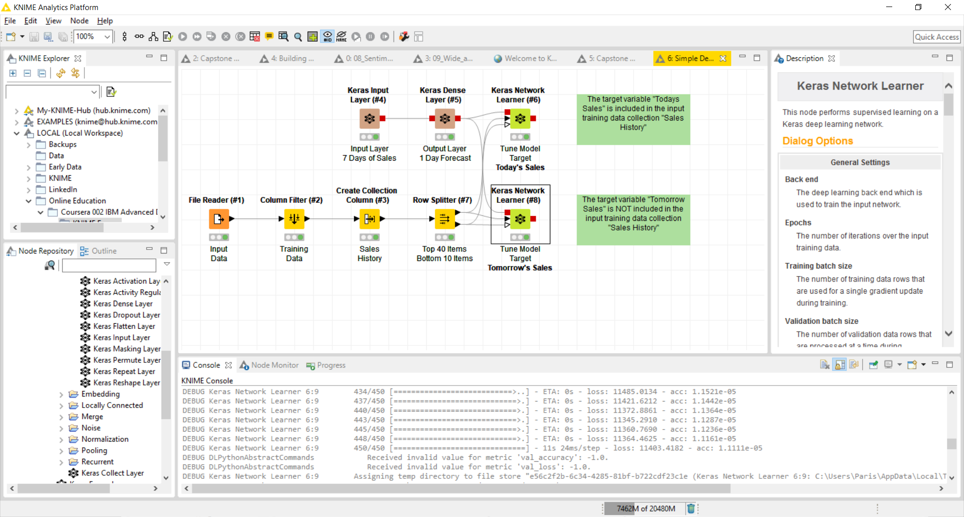
I’m trying to reproduce my Python Keras neural networks in KNIME and I can’t even get a simple feed-forward network to tune.

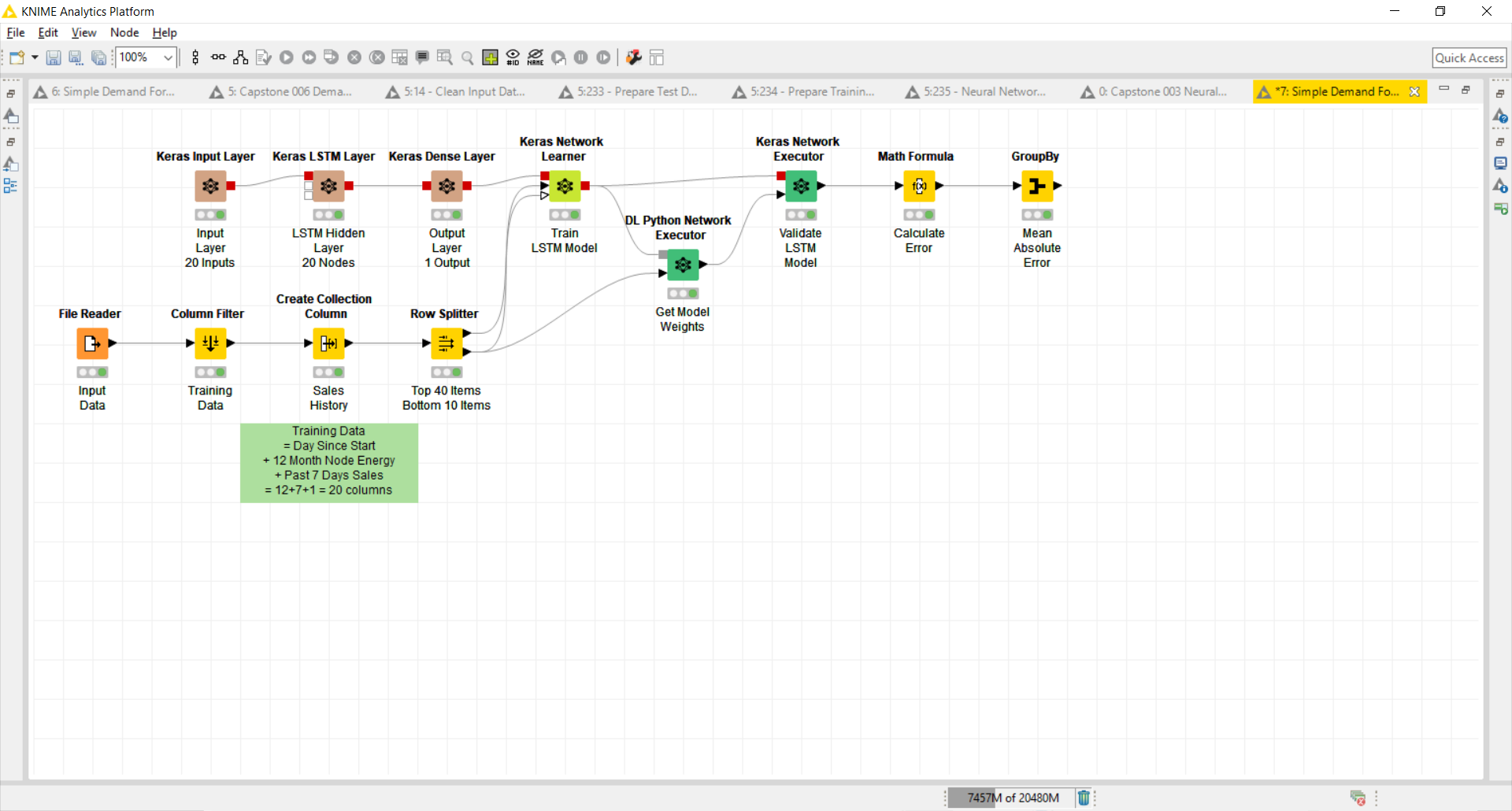
I’ve started with a traditional 3-layer neural network comprising of the following layers:

• Input Layer
• Hidden Layer (implied)
• Output Layer

I’ve pulled historic sales data from a Kaggle challenge (https://www.kaggle.com/c/demand-forecasting-kernels-only/data) and I’m trying to train this neural network to recognize weekly sales trends. That is, I want the model to recognize that last Monday’s sales are proportional to this Monday’s sales. I’ve got 7 input nodes (each with sales data from the last 7 days) and 1 output node (used to predict the sales for tomorrow). Once I get things working I’d like to train the model to recognize seasonality as well as year-over-year growth.

To test the network I’ve made it even easier by asking the neural network to predict today’s sales, where today’s sales are actually passed within the last 7 days of data.

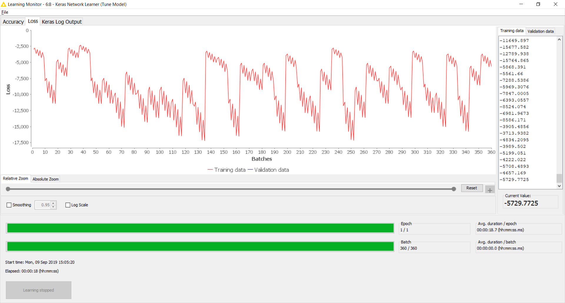
But my results are horrendous!

The log from the Learning Monitor for [target = Today] looks like this:

Epoch 1/1

  1/360 [..............................] - ETA: 1:12 - loss: 41.1427 - acc: 0.0050
  6/360 [..............................] - ETA: 15s - loss: 1308.4251 - acc: 8.3333e-04
  9/360 [..............................] - ETA: 12s - loss: 1380.3868 - acc: 5.5556e-04
 12/360 [>.............................] - ETA: 11s - loss: 3253.8582 - acc: 4.1667e-04
 15/360 [>.............................] - ETA: 10s - loss: 5183.7564 - acc: 3.3333e-04
 17/360 [>.............................] - ETA: 10s - loss: 6294.8577 - acc: 2.9412e-04
 20/360 [>.............................] - ETA: 9s - loss: 6610.1236 - acc: 2.5000e-04 
 23/360 [>.............................] - ETA: 9s - loss: 6184.6507 - acc: 2.1739e-04
 26/360 [=>............................] - ETA: 9s - loss: 6232.6921 - acc: 1.9231e-04
 28/360 [=>............................] - ETA: 9s - loss: 6035.7421 - acc: 1.7857e-04
 31/360 [=>............................] - ETA: 8s - loss: 5638.0236 - acc: 1.6129e-04
 32/360 [=>............................] - ETA: 9s - loss: 5464.3688 - acc: 1.5625e-04
 35/360 [=>............................] - ETA: 8s - loss: 5203.6640 - acc: 1.4286e-04
 38/360 [==>...........................] - ETA: 8s - loss: 4900.0533 - acc: 1.3158e-04
 41/360 [==>...........................] - ETA: 8s - loss: 4603.7346 - acc: 1.2195e-04
 44/360 [==>...........................] - ETA: 8s - loss: 4405.1444 - acc: 1.1364e-04
 47/360 [==>...........................] - ETA: 8s - loss: 4480.1594 - acc: 1.0638e-04
 50/360 [===>..........................] - ETA: 8s - loss: 4743.8953 - acc: 1.0000e-04
 53/360 [===>..........................] - ETA: 7s - loss: 5436.0964 - acc: 9.4340e-05
 55/360 [===>..........................] - ETA: 7s - loss: 5715.3838 - acc: 9.0909e-05
 59/360 [===>..........................] - ETA: 7s - loss: 5987.4896 - acc: 8.4746e-05
 61/360 [====>.........................] - ETA: 7s - loss: 6137.9276 - acc: 8.1967e-05
 64/360 [====>.........................] - ETA: 7s - loss: 6749.1277 - acc: 7.8125e-05
 67/360 [====>.........................] - ETA: 7s - loss: 7116.1035 - acc: 7.4627e-05
 69/360 [====>.........................] - ETA: 7s - loss: 7593.8689 - acc: 7.2464e-05
 72/360 [=====>........................] - ETA: 7s - loss: 8103.8618 - acc: 6.9444e-05
 75/360 [=====>........................] - ETA: 7s - loss: 8307.9650 - acc: 6.6667e-05
 78/360 [=====>........................] - ETA: 7s - loss: 8440.0061 - acc: 6.4103e-05
 81/360 [=====>........................] - ETA: 7s - loss: 8445.4454 - acc: 6.1728e-05
 84/360 [======>.......................] - ETA: 7s - loss: 8799.0436 - acc: 5.9524e-05
 87/360 [======>.......................] - ETA: 6s - loss: 9094.5771 - acc: 5.7471e-05
 90/360 [======>.......................] - ETA: 6s - loss: 9409.4286 - acc: 5.5556e-05
 93/360 [======>.......................] - ETA: 6s - loss: 9734.1981 - acc: 5.3763e-05
 96/360 [=======>......................] - ETA: 6s - loss: 9980.4404 - acc: 5.2083e-05
 98/360 [=======>......................] - ETA: 6s - loss: 10204.8440 - acc: 5.1020e-05
100/360 [=======>......................] - ETA: 6s - loss: 10370.7380 - acc: 5.0000e-05
103/360 [=======>......................] - ETA: 6s - loss: 10467.4699 - acc: 4.8544e-05
105/360 [=======>......................] - ETA: 6s - loss: 10624.3502 - acc: 4.7619e-05
108/360 [========>.....................] - ETA: 6s - loss: 10754.4471 - acc: 4.6296e-05
110/360 [========>.....................] - ETA: 6s - loss: 10957.5650 - acc: 4.5455e-05
113/360 [========>.....................] - ETA: 6s - loss: 11366.7011 - acc: 4.4248e-05
116/360 [========>.....................] - ETA: 6s - loss: 11862.1118 - acc: 4.3103e-05
118/360 [========>.....................] - ETA: 6s - loss: 11987.4646 - acc: 4.2373e-05
121/360 [=========>....................] - ETA: 6s - loss: 11999.5912 - acc: 4.1322e-05
124/360 [=========>....................] - ETA: 5s - loss: 11925.4825 - acc: 4.0323e-05
126/360 [=========>....................] - ETA: 5s - loss: 12003.1657 - acc: 3.9683e-05
129/360 [=========>....................] - ETA: 5s - loss: 12310.0577 - acc: 3.8760e-05
132/360 [==========>...................] - ETA: 5s - loss: 12622.5914 - acc: 3.7879e-05
133/360 [==========>...................] - ETA: 5s - loss: 12671.4426 - acc: 3.7594e-05
137/360 [==========>...................] - ETA: 5s - loss: 12898.7462 - acc: 3.6496e-05
140/360 [==========>...................] - ETA: 5s - loss: 12759.9382 - acc: 3.5714e-05
143/360 [==========>...................] - ETA: 5s - loss: 12552.1473 - acc: 3.4965e-05
146/360 [===========>..................] - ETA: 5s - loss: 12340.1664 - acc: 3.4247e-05
149/360 [===========>..................] - ETA: 5s - loss: 12175.1636 - acc: 3.3557e-05
151/360 [===========>..................] - ETA: 5s - loss: 12061.2759 - acc: 3.3113e-05
154/360 [===========>..................] - ETA: 5s - loss: 11994.9607 - acc: 3.2468e-05
156/360 [============>.................] - ETA: 5s - loss: 12077.8994 - acc: 3.2051e-05
159/360 [============>.................] - ETA: 5s - loss: 12353.0585 - acc: 3.1447e-05
163/360 [============>.................] - ETA: 4s - loss: 12623.3139 - acc: 3.0675e-05
166/360 [============>.................] - ETA: 4s - loss: 12537.7248 - acc: 3.0120e-05
168/360 [=============>................] - ETA: 4s - loss: 12462.8419 - acc: 2.9762e-05
171/360 [=============>................] - ETA: 4s - loss: 12333.8680 - acc: 2.9240e-05
174/360 [=============>................] - ETA: 4s - loss: 12267.9013 - acc: 2.8736e-05
177/360 [=============>................] - ETA: 4s - loss: 12190.9796 - acc: 2.8249e-05
179/360 [=============>................] - ETA: 4s - loss: 12167.1833 - acc: 2.7933e-05
182/360 [==============>...............] - ETA: 4s - loss: 12073.5335 - acc: 2.7473e-05
186/360 [==============>...............] - ETA: 4s - loss: 11934.0249 - acc: 2.6882e-05
189/360 [==============>...............] - ETA: 4s - loss: 11824.2404 - acc: 2.6455e-05
192/360 [===============>..............] - ETA: 4s - loss: 11940.1421 - acc: 2.6042e-05
194/360 [===============>..............] - ETA: 4s - loss: 12013.8136 - acc: 2.5773e-05
198/360 [===============>..............] - ETA: 3s - loss: 12227.3909 - acc: 2.5253e-05
200/360 [===============>..............] - ETA: 3s - loss: 12244.4892 - acc: 2.5000e-05
203/360 [===============>..............] - ETA: 3s - loss: 12136.9278 - acc: 2.4631e-05
206/360 [================>.............] - ETA: 3s - loss: 12018.5440 - acc: 2.4272e-05
209/360 [================>.............] - ETA: 3s - loss: 11952.3829 - acc: 2.3923e-05
212/360 [================>.............] - ETA: 3s - loss: 11968.1454 - acc: 2.3585e-05
215/360 [================>.............] - ETA: 3s - loss: 12084.7486 - acc: 2.3256e-05
218/360 [=================>............] - ETA: 3s - loss: 12107.6915 - acc: 2.2936e-05
221/360 [=================>............] - ETA: 3s - loss: 12289.4988 - acc: 2.2624e-05
224/360 [=================>............] - ETA: 3s - loss: 12489.4115 - acc: 2.2321e-05
227/360 [=================>............] - ETA: 3s - loss: 12525.3862 - acc: 2.2026e-05
230/360 [==================>...........] - ETA: 3s - loss: 12428.8609 - acc: 2.1739e-05
233/360 [==================>...........] - ETA: 3s - loss: 12422.4053 - acc: 2.1459e-05
235/360 [==================>...........] - ETA: 3s - loss: 12351.1595 - acc: 2.1277e-05
237/360 [==================>...........] - ETA: 2s - loss: 12281.3554 - acc: 2.1097e-05
239/360 [==================>...........] - ETA: 2s - loss: 12192.0119 - acc: 2.0921e-05
243/360 [===================>..........] - ETA: 2s - loss: 12020.3736 - acc: 2.0576e-05
246/360 [===================>..........] - ETA: 2s - loss: 12069.1666 - acc: 2.0325e-05
249/360 [===================>..........] - ETA: 2s - loss: 12303.1701 - acc: 2.0080e-05
252/360 [====================>.........] - ETA: 2s - loss: 12436.7261 - acc: 1.9841e-05
256/360 [====================>.........] - ETA: 2s - loss: 12601.9745 - acc: 1.9531e-05
258/360 [====================>.........] - ETA: 2s - loss: 12640.4291 - acc: 1.9380e-05
261/360 [====================>.........] - ETA: 2s - loss: 12667.2074 - acc: 1.9157e-05
263/360 [====================>.........] - ETA: 2s - loss: 12686.5048 - acc: 1.9011e-05
266/360 [=====================>........] - ETA: 2s - loss: 12595.4022 - acc: 1.8797e-05
269/360 [=====================>........] - ETA: 2s - loss: 12541.3375 - acc: 1.8587e-05
273/360 [=====================>........] - ETA: 2s - loss: 12491.4365 - acc: 1.8315e-05
276/360 [======================>.......] - ETA: 2s - loss: 12481.2461 - acc: 1.8116e-05
279/360 [======================>.......] - ETA: 1s - loss: 12464.7419 - acc: 1.7921e-05
281/360 [======================>.......] - ETA: 1s - loss: 12466.3107 - acc: 1.7794e-05
284/360 [======================>.......] - ETA: 1s - loss: 12383.0751 - acc: 1.7606e-05
286/360 [======================>.......] - ETA: 1s - loss: 12347.9585 - acc: 1.7483e-05
289/360 [=======================>......] - ETA: 1s - loss: 12346.7884 - acc: 1.7301e-05
292/360 [=======================>......] - ETA: 1s - loss: 12348.0108 - acc: 1.7123e-05
295/360 [=======================>......] - ETA: 1s - loss: 12396.0276 - acc: 1.6949e-05
297/360 [=======================>......] - ETA: 1s - loss: 12428.4331 - acc: 1.6835e-05
301/360 [========================>.....] - ETA: 1s - loss: 12360.6918 - acc: 1.6611e-05
304/360 [========================>.....] - ETA: 1s - loss: 12259.6471 - acc: 1.6447e-05
306/360 [========================>.....] - ETA: 1s - loss: 12194.8393 - acc: 4.9020e-05
310/360 [========================>.....] - ETA: 1s - loss: 12196.0194 - acc: 4.8387e-05
312/360 [=========================>....] - ETA: 1s - loss: 12218.6873 - acc: 4.8077e-05
316/360 [=========================>....] - ETA: 1s - loss: 12301.3521 - acc: 4.7468e-05
319/360 [=========================>....] - ETA: 0s - loss: 12332.4387 - acc: 4.7022e-05
321/360 [=========================>....] - ETA: 0s - loss: 12401.6317 - acc: 4.6729e-05
324/360 [==========================>...] - ETA: 0s - loss: 12458.0278 - acc: 4.6296e-05
327/360 [==========================>...] - ETA: 0s - loss: 12453.6503 - acc: 4.5872e-05
329/360 [==========================>...] - ETA: 0s - loss: 12393.3611 - acc: 4.5593e-05
332/360 [==========================>...] - ETA: 0s - loss: 12315.8433 - acc: 4.5181e-05
335/360 [==========================>...] - ETA: 0s - loss: 12299.0822 - acc: 4.4776e-05
336/360 [===========================>..] - ETA: 0s - loss: 12320.2354 - acc: 4.4643e-05
339/360 [===========================>..] - ETA: 0s - loss: 12426.3547 - acc: 4.4248e-05
343/360 [===========================>..] - ETA: 0s - loss: 12538.7709 - acc: 4.3732e-05
345/360 [===========================>..] - ETA: 0s - loss: 12509.6730 - acc: 4.3478e-05
348/360 [============================>.] - ETA: 0s - loss: 12468.1871 - acc: 4.3103e-05
350/360 [============================>.] - ETA: 0s - loss: 12444.8846 - acc: 4.2857e-05
352/360 [============================>.] - ETA: 0s - loss: 12402.9514 - acc: 4.2614e-05
355/360 [============================>.] - ETA: 0s - loss: 12325.5229 - acc: 4.2254e-05
358/360 [============================>.] - ETA: 0s - loss: 12241.9661 - acc: 4.1899e-05
360/360 [==============================] - 13s 37ms/step - loss: 12194.5712 - acc: 4.1667e-05 - val_loss: 10412.9327 - val_acc: 0.0000e+00

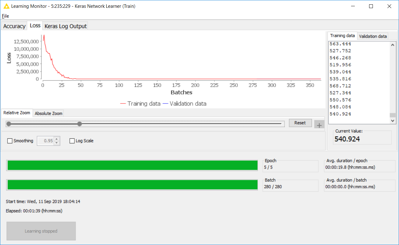
On the other hand, the results I get from Python look ok (Python is running in IBM Watson Studio - not within KNIME).

My node weights from Python for [target = Today] look like this:

Sales(-6) = 0.0000
Sales(-5) = 0.0001
Sales(-4) = 0.0001
Sales(-3) = 0.0000
Sales(-2) = -0.0001
Sales(-1) = 0.0000
Sales(0) = 0.7391

Conclusion: the Python network correctly predicted that today’s sales is proportional to sales from day 0 (that is, sales from today).

And my node weights from Python for [target = Tomorrow] look like this:

Sales(-6) 1.0840
Sales(-5) -0.0591
Sales(-4) 0.0850
Sales(-3) 0.0487
Sales(-2) -0.1068
Sales(-1) 0.0940
Sales(0) 0.2058

Conclusion: Again, the Python network correctly predicted that tomorrow’s sales is proportional to sales from Sales(-6) (that is, sales from 7 days ago).

What am I doing wrong with KNIME?

Additional Question #1: Is there a way to see the compiled Neural Network topology from within KNIME (similar to the Python model.summary() command)?

Additional Question #2: Is there a way to see individual node tuning weights from within KNIME (similar to the Python layer.get_weights() command)?

Simple Demand Forecast Neural Network 001.knwf (3.4 MB)

[nemad]

Hello @Edlueze,

a couple of things I noticed in your workflow:

• The option to shuffle the data is disabled, is that intended? Shuffling usually helps to prevent oscillations and can stabilize training (if I am not mistaken, Keras does it by default).
• You are using Stochastic Gradient Descent as optimizer. Playing a bit with the learning rate I found that the learning rate of 0.01 is too large and a smaller learning rate is required. I also found that e.g. Adam delivers considerably better results with its default configuration.
• In the second learner, the loss function is set to Binary Cross Entropy but I guess it should be mean absolute error (or some loss for regression) instead.

Regarding Additional Question #1:
If you open the network port of a node outputing a Keras Network, you can browse through the different layers.

Regarding Additional Question #2:
No this is currently not directly supported but you can use the Python command in the DL Python Network Executor node. You just need to set a dummy input table which you ignore in the script.

Cheers,

Adrian

[Edlueze]

Thanks Adrian @nemad - very useful!

When developing with Python I only needed to worry about a couple of parameters. But when trying to replicate the same results with the KNIME Keras nodes, all of the inputs were exposed and I found myself floundering in a sea of configuration options. A sanity check was exactly what I needed.

Thanks to your suggestions, I’ve had a fun day building a comparison between the Keras Layer nodes and the DL Python nodes. I finally got the two model workflows to agree. Keeping the networks simple has been really helpful as it was easy to look at the weights and see if the networks were acting as expected. There are some great advanced neural network examples on KNIME Hub, but I see a need for a super simple one like this one - so I’m going to polish it up and post it for the community. Stay tuned!

My next step is to expand the analysis to pick up on longer term trends in the sales history: namely seasonality and year-over-year growth. I’m going to need to add more input nodes and more hidden layers, and maybe even try an LSTM recurrent neural network.

Perhaps you, or another expert, might have some advice on these more general neural network questions:

Question 1: I’d like to add a non-linear activation function to the network, but I’m worried about the sigmoid function as my final output isn’t going to be between 0.0 and 1.0. Even if a downstream layer could re-scale the predictions back up, is it sensible to run all the analysis through such a truncation? A parallel branching network might solve this problem but also might be overkill. Any suggestions?

Question 2: If I’ve already got the last 7-days of data coming in as input nodes, does it even make sense to use an LSTM model?

Ted.

[nemad]

Hi Ted,

I am happy to hear the deep learning integration now works for you and I am looking forward to your workflow on the hub.
Regarding your questions:

1. In order to learn non-linear functions, a deep learning network needs non-linear activation functions because many linear layers, in the end, will also just represent a linear function. However, for hidden activations sigmoid is rarely used nowadays because it can cause the vanishing gradient problem. Instead, people now usually use ReLU or Leaky ReLU.

2. For your use-case above, an LSTM is probably not much better than the dense model you have right now. However, if you consider longer time-series (e.g. the last 30 days) with multiple features per time-step (e.g. demand and temperature), an LSTM will quickly start to outperform a dense model.

Cheers,

Adrian

[Edlueze]

For those interested in seeing these simple demand forecasting neural networks, you can download the workflow from the KNIME Hub:

https://hub.knime.com/scientificstrategy/space/KNIME%20Nodes/KN-301%20Simple%20Demand%20Forecasting%20Neural%20Networks%20v03

For step-by-step instructions, visit this blog:

https://scientificstrategy.com/kn-301/

[Edlueze]

Hi Adrian @nemad - it looks like I am not out of trouble yet. I’m now trying to implement an LSTM model and can’t get any results.

Simple Demand Forecast Neural Network 003.knwf (2.0 MB)

As you suggested, I’m now using the last 30 days of sales data. I’ve also added a “Periodic Encoding” feature to each row to help the model with monthly seasonality. My reasoning is as follows:

Because the data contains seasonality, it is necessary to help the Neural Network identify the season from which the data comes. A simple way to do this would be to one-hot encode the months - that is, turn on 1 of 12 input nodes. But this approach is flawed as the Neural Network would have no way of knowing that December (12) is near January (1). Or, for that matter, that February and January are adjacent. Instead, the “Periodic Encoding” method applies some energy to each of the 12 month nodes depending upon how close the training day is to the month.

For example, if training the data from June-15 then the “June” node would be turned completely on (set to 1.0) with “May” and “July” nodes also receiving some energy (set to 0.6). The more distant months “April” and “August” get less energy still (set to 0.15). If training the data from the start of Jan-01 then January would not be completely turned on (being set to only 0.9). As December just finished it would receive almost as much (set to 0.88). But February would receive much less (0.35).

The LSTM model I’ve created is not much more complicated than the earlier Feed Forward model, and the model does seem to be updating the weights. But the model predicts that future sales will all be zero.

Any help would be appreciated!

PS I’ve simplified the model by reducing the data down to the last 7-days in the attached example. I’ve also tried shuffling and unshuffling. Shuffled tuning looks slightly better, but I though LSTM models always had to use unshuffled data within a batch.

Simple Demand Forecast Neural Network 003.knwf (2.0 MB)

[Edlueze]

Update: Normalizing all of the input data is helping. And it makes sense - the neural network isn’t going to be able to handle input data on very different scales with random initialization to the weights.

But tuning is now much slower, and the results still seem much worse than the simple Feed Forward model. Also, I really wanted the model to identify the year-over-year sales growth. But if I normalize the data then I worry that this growth input will disappear.

Your help would still be appreciated!

[nemad]

Hello Ted,

for an LSTM you will have to model your input differently, i.e. as a real sequence.
Currently, your input represents a time series with only a single time step that contains the past time steps as one of its twenty features.
For an LSTM to work properly, you would have to model it so that you have for each of the past 7 days 14 features (the 12 energies, day since start and the sales of that day).
Your input then would have the shape [7, 14] instead of [1, 20] which corresponds to a sequence of 7 days.
I have to admit that the handling of inputs of this shape is somewhat awkward and I am not sure if it actually helps the network too much to have the energies for every of the past 7 days since that information is contained in the energies for the present day.
Therefore I’d suggest to model it slightly differently, i.e. you use an LSTM to analyze the sequence of past sales and have an additional input layer that receives the day since start and the energies.
You then concatenate the output of the LSTM with the additional input and predict the output with a dense layer.

Some more thoughts:

• The periodic encoding looks interesting.
• In your LSTM layer, the activations are set to ReLU, I know, I said that sigmoid is no longer used for hidden activations but the LSTM is an exception to that rule because it uses sigmoids to model gates through which information can be added or removed to the state of the layer
• There are almost no cases, where shuffling is not recommended. What you have to keep in mind for sequence analysis is that the order within a single example may not change, though. That means you can’t shuffle the past 7 days in your example.
• Normalization plays a critical role since the magnitude of the features directly influences the model outputs, so to give all features equal influence on the model, they should roughly be on the same scale.
• In case of sequence data normalization is perhaps more tricky because you have to normalize all sales columns with the same transformation.
• The slower convergence you observed is because smaller features mean smaller activations which in turn (depending on your architecture) mean smaller gradients and the magnitude of the gradient is tied to the magnitude of updates to the waits. A remedy could be to increase the learning rate but not so much that the model starts diverging (i.e. the loss grows instead of shrinks).

Cheers,

Adrian

[Edlueze]

Thanks Adrian - very useful!

After a week’s distraction I am getting back to this. The models have been running well and I’m now working on the refinements you’ve suggested.

Silly question - why is my ‘Accuracy’ in the ‘Learning Monitor’ always zero regardless of network type? Only the ‘Loss’ tab in the ‘Learning Monitor’ shows anything. I suspect it’s because I haven’t defined an accuracy function (only a loss function). But how do you do that???

[nemad]

Hi Ted,

that is because the accuracy is only well-defined for classification problems.
Unfortunately, it is not yet possible to select any other metric but in case of regression problems the loss usually is already a good metric for the model quality.

Cheers,

Adrian

[Edlueze]

I just posted the more advanced sales forecasting neural network workflow on KNIME Hub:

Sales Demand Forecasting Neural Networks

This contains the reset workflow. If you want more details and the un-reset workflow (over 400 MB) then you can download it from here:

KN-302 Advanced Demand Forecast Neural Networks

[nemad]

Hi Ted,

awesome work!
Thank you for sharing it with the KNIME community

Best regards,

Adrian