This course introduces the main concepts behind Time Series Analysis, with an emphasis on forecasting applications: data cleaning, missing value imputation, time-based aggregation techniques, creation of a vector/tensor of past values, descriptive analysis, model training (from simple basic models to more complex statistics and machine learning based models), hyperparameter optimization, and model evaluation.
Learn how to implement all these steps using real-world time series datasets. Put what you’ve learnt into practice with the hands-on exercises.
This course consists of 4 x 90-minute online sessions run by Professor Daniele Tonini and two of our KNIME data scientists. Each session has an exercise for you to complete at home. The course concludes with a 15 to 30-minute wrap-up session.
Course Content
Session 1: Introduction to Time Series Analysis and KNIME Components
Session 2: Understanding Stationarity, Trend and Seasonality
I enjoyed the first session quite alot and I’m looking forward to the deep dives!
Out of curiosity:
Is there a plan to develop the time series nodes as generic KNIME nodes, as well? What is the advantage of using components rather than programming them as generic nodes?
Personally, I am used to python, but it is always a bit cumbersome when introducing colleagues to a low coding tool KNIME and then explain that they would also need to install scripting libraries for certain features
In the long term we hope to provide more and more time series functionalities as KNIME native nodes. In the short term, we’re developing and enhancing our time series components.
Components are KNIME nodes that encapsulate functionalities built by other KNIME nodes. For a data scientist, building a workflow or writing a script is often easy, but some other types of users prefer a component with clearly defined task and configuration settings in the configuration dialog. On the other side, if you’d like to, you can also customize the functionalities of the components. For example, you as a Python programmer could add functionalities to our time series components that are based on Python code.
You’re right, it’s not ideal at the moment that the Python libraries need to be installed separately. But at the moment this is required to excute Python code from within KNIME without writing any code.
The one-pager for setting up the python environment is very useful. It is probably beyond the scope of this great course, but would TSA with R require a similar setup? If so, is there such a one-pager or cheat sheet available for using R?
Hi Thomas, this is because not all techniques for missing value handling available in the missing value node can be exported as PMML (the model output of the node). If you configured the node to use such a technique, you will get this notification, but it’s only a warning, not an error.
Hi Thomas, many Windows users say integrating R statistics in KNIME is more straightforward than integrating Python, and indeed it requires fewer steps, with the local installation of R and Rserve package installed. You can check the required steps for installing R Statistics Integration in KNIME on this documentation page: https://docs.knime.com/2019-12/r_installation_guide/index.html
ARIMA Modelling:
About decomposing a time series, what would be the best strategy here? Decompose it myself or just let ARIMA do the job? My first impression is that an automated ARIMA (learner) does a much better job here? Manual decomposition would be rather a technique to analyze the time series and describe it?
Models for heteroskedasticity:
ARIMA does not assume shocks in other statistical moments, e.g. Variance, am I right? The ARCH model “zoology” would come into play here. Are there also components covering ARCH processes? But similar to the ARIMA universe, one could just use ML and Deep Learning models for these cases as well?
Components in general (off topic):
If a component gets uploaded by the community to the hub, is there a kind of quality gate, that tests the component for functionality and also for the theory behind it?
Machine Learning & Deep Learning:
Also my (beginner’s) first impression about ML is, that ML beats classical models by haveing a better fit to the data and also much less restrictions / assumptions when implementing them. What speaks for classical models, such as ARIMA then? I guess one point would be the analytical traceability? Are there cases where classical and parsimonious models beat ML models?
Deep Learning (maybe a more philosophical question):
The power of DL is quite impressive. However, analytical traceability is limited here. I am a little bit worried about users/colleagues (including myself) using it negligently and forming false conclusions about the reality by trusting DL algorithms too much. What would be here the best strategy, when to apply Deep Learning techniques? For example, if the DL model performs only slightly better than a parsimonious ML model, wouldn’t it be more reasonable to go with the parsimonious model, where analytics and math behind the model can be better understood?
Thanks a lot for the great sessions. They were really insightful!
Hi, here answers to your questions. We’re happy to elaborate them in today’s Q&A session if needed.
ARIMA Modeling
ARIMA models assume stationary series, and therefore we first manually decompose the series into a trend, first and second seasonalities, and residual, which is supposed to be stationary. ARIMA model can only make a time series stationary by first order differencing (I order 1), maximum two times (I order 2), but it cannot perform the seasonal differencing like we perform manually at lags 24 and 168. Besides that, the manual decomposition is also used to inspect and describe the time series.
Models for heteroscedasticity
Unfortunately, we don’t have components for ARCH models
Components in general
Components uploaded by the KNIME community are not quality checked by KNIME. Components uploaded by KNIME (those also available on the EXAMPLES Server) are tested regularly.
Machine Learning & Deep Learning
Classical models often work the best with small amounts of data available, and with frequent changes in the data
Deep Learning
Deep learning techniques have the disadvantage of low interpretability and slow computation. If these are not an issue in your use case, the deep learning model might be the right choice. However, like you said, the highest accuracy is not always the most important criterion when selecting a model. Deep learning models also require a lot of training data to perform well. If you have a time series with frequently changing dynamics, enough training data are often not available.
@Maarit: Thanks alot for the answers! Things became much clearer now.
I had the chance now to put the components into action and few more questions popped up.
Is there a possibility to check if a timeseries itself is stationary? A common statistical tool would be the (augmented) dickey fuller test. Is there an ADF node already available?
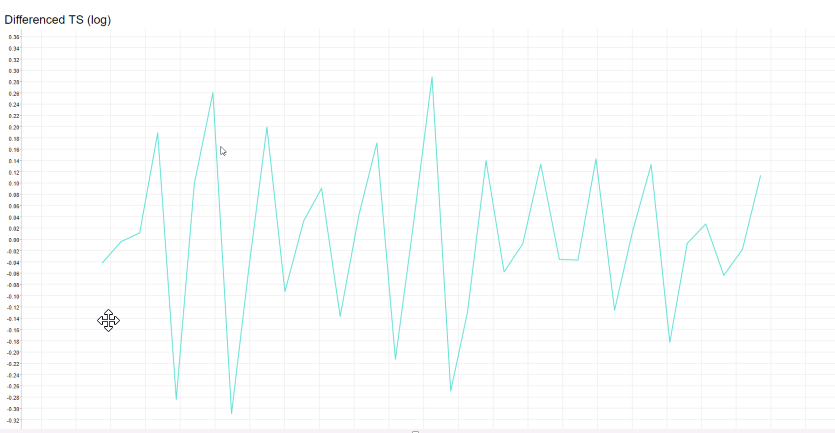
I have a time series, which I log differenced and it looks quite stationary to me:
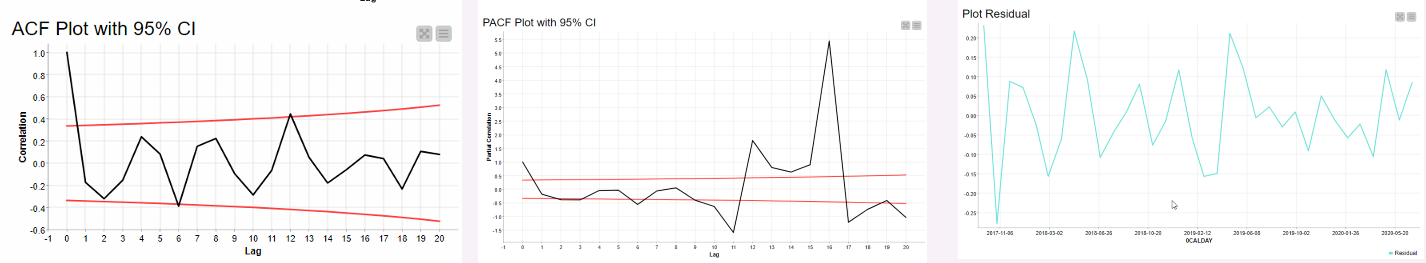
I applied the decompose node to further reduce seasonality and trend and ACF and PACF decay initially into the 95% CI Bounds. What worries me a little is the PACF spike at leg 11, 12 and 16. How can I interpret it and do I have to remove it before applying ARIMA? And how could I remove it? See screen below (left ACF, middle PACF and right residual plot -> residual after decomposing)
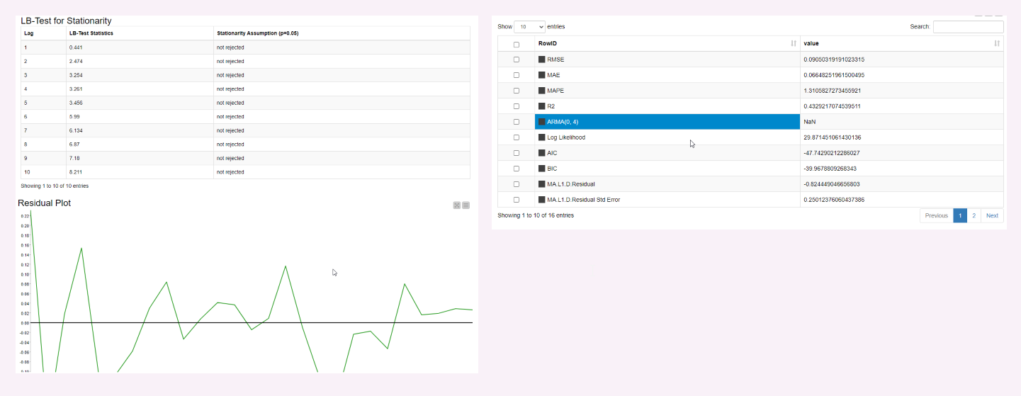
Let’s assume the time series is optimal for ARIMA modelling and the auto Arima Model suggests the best fit Model. In my case this is an ARMA (0,4) and the ARIMA residuals are stationary (see screen below).
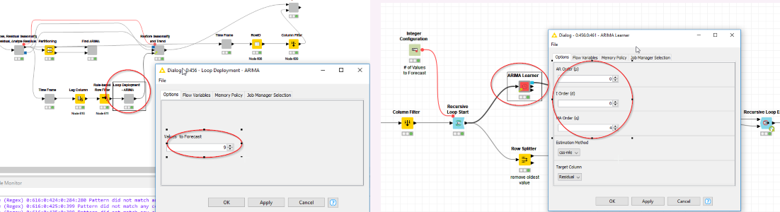
My approach for deployment would be to take the Hyper Parameters of the ARIMA Learner (ARMA 0,4) and enter them into ARIMA Learner within the loop deployment metanode. My question: Since I have initially (log) differenced the time series to make it stationary, do I have to enter also the integration Hyperparameter I=1 into the ARIMA learner for deployment, i.e. ARIMA (0,1,4), or is this already considered and I just have to enter ARMA (0,4), which the auto ARIMA learner suggests?
Sometimes it seems that the ARIMA learner wants me to enter a Hyperparameter I, even though I have differenced the timeseries before and I get the error message listed here:
And last question so far: For the ARIMA Learner, it sometimes happens that I get the error message:
numpy.linalg.LinAlgError: SVD did not converge
I found this post, however, I cannot imagine where “NaN” or “inf” values would appear. Do you know more about this error message?
Thanks again for your support! I hope the questions are not to much of a hassle. If there are any unclear points, feel free to reach out
Thank you for your questions. It’s nice to see that you’re using our time series components.
You can use the Analyze ARIMA residuals component to check the stationarity of any time series, not only the residuals of an ARIMA model. Unfortunately, this component only implements the Ljung-Box test and not the ADF test.
Let me ask Daniele about this
ARIMA model only needs the I parameter if the time series should be differenced to make it stationary. If the log differenced time series is stationary, then the I parameter should be 0. If the model requires a non-zero I parameter, then the log differenced time series is probably not stationary.
Let me ask Corey about this
I’ll come back to you with more answers as soon as possible. Sorry for the late reply.
Regarding the second question, Daniele pointed out the following aspects:
The significant lags in the PACF plot might indicate over-differencing.
What is the granularity of the data. 16 is a pretty old lagged value.
The values of partial correlation are strange too, as they are higher than 1. This can happen (depending on the algorithm used to estimate the PACF function) when you have few obs… in this case, the partial autocorrelation values for the highest lags are not reliable (few degrees of freedom left to estimate them).
Would it be possible to see the ACF/PACF plots before and after each transformation step, or could you share the workflow?
And regarding the Python error: The model is not converging for some reason. It could be that if you’re using two years of monthly data (this is how the ACF plot looks like) it might not be enough data to build an ARIMA model. We’re working on a more informative error message, though. Thank you for mentioning this!
To add something of my experience.
When I was following the descriptions in Forecasting: Principles and Practice by Rob J Hyndman and George Athanasopoulos (which is based on R instead of Python; but the principles are the same) I ran into issues as well when I tried to use either an X11-decomposition or SEATS decomposition (Seasonal Extraction in ARIMA Time Series).
For both methodes a minimum of 40 data points, i.e. 40 months in your case, is required, otherwise they will not work.
At the 2020 Fall Summit during the Time Series Training, there was talk about new Components that can handle Seasonality. Do we have a rough expected time frame for beta release? If no, I will have some questions about how to add back the seasonality for value prediction.
Trying to create a view like this, where the light blue in the plot shows the 95% confidence interval, and the dark blue shows the 80% confidence interval:
We showed a preliminary version of the SARIMA component in the course, which you can use to create forecasts of data with seasonal patterns. We are actively working on it, but I can’t promise anything about the release. I hope soon!
The ARIMA Predictor component outputs the standard deviations of the out-sample predictions. You can use these values to calculate the 80% and 95% confidence bounds, and plot them together with the predictions in the same line plot. After restoring the seasonality and trend to your ARIMA predictions and their confidence bounds, the lines should look pretty similar to the one you show in the view.
Unfortunately I don’t know about any KNIME resources for time series analysis in R. But in the course slides we reference this book which was used by Prof. Daniele Tonini who is a creator of the course.