This workflow shows the seasonality of time series (energy consumption) in an autocorrelation plot. The seasonality is removed by differencing the time series at the lag where the maximum peak is detected in the autocorrelation plot. As an alternative approach, the time series is decomposed into its trend, first and second seasonalities, and irregular component. The distribution of energy consumption for each hour is shown for both the original and differenced time series.
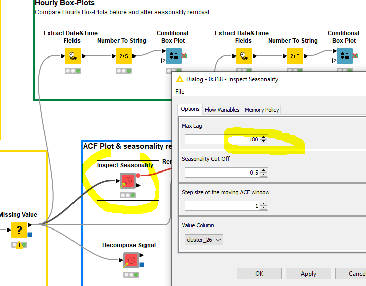
It’s somewhat arbitrary, but I believe the idea here is that you want to set a max lag that would cover a “reasonable” amount of seasonality that you might expect to see. Since this is hourly data, a lag of 180 goes back approximately 1 week.
Dear @ScottF ,
As I posted in greater detail at < Autocorrelation and Seasonality in Time Series >, I am facing a somewhat comparable situation.
Notwithstanding, I could not install Python (or its libraries) on my PC. Therefore, I could not apply any suggestion similar to the one depicted in this post. So, I ask you if you might help me with a solution (in Knime, but without Python or R) to my problem, as stated in the forum (link above).
Thank you for any help.
B.R.,
Rogério.