H2O.ai Automl - a powerful auto-machine-learning framework wrapped with KNIME
It features various models like Random Forest or XGBoost along with Deep Learning. It has wrappers for R and Python but also could be used from KNIME. The results will be written to a folder and the models will be stored in MOJO format to be used in KNIME (as well as on a Big Data cluster via Sparkling Water).
One major parameter to set is the running time the model has to test various models and do some hyperparameter optimization as well. The best model of each round is stored, and some graphics are produced to see the results.
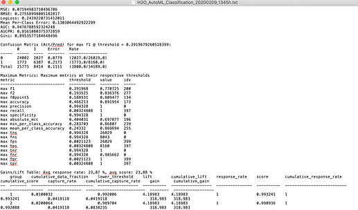
Results are interpreted through various statistics and model characteristics are stored in an Excel und TXT file as well as in PNG graphics you can easily re-use in presentations and to give your winning models a visual inspection.
Also, you could use the Meta node “Model Quality Classification - Graphics” to evaluate other binary classification models:
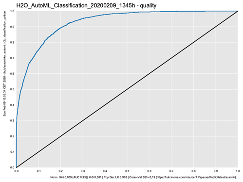
ROC Curve and Gini coefficient
A classic ROC (receiver operating characteristic) curve with statistics like the Gini coefficient measuring the ‘un-equality’ – which is what we want to maximize in this case
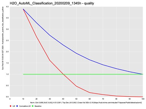
TOP Decile Lift
A classic lift curve with statistics. Illustrating how the TOP 10% of your score is doing compared to the rest. You have the cumulative lift that ends in 1.0 (the green line ^= the average % of Targets in your population) and the Lift for each 10% step. This graphic and statistics are useful if you want to put emphasis on the Top group.
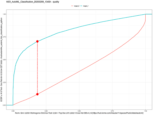
Kolmogorov-Smirnov Goodness-of-Fit Test
two curves illustrating the Kolmogorov-Smirnov Goodness-of-Fit Test. An indication of how good the two groups have been separated. The higher the better. Also, inspect the curves visually.
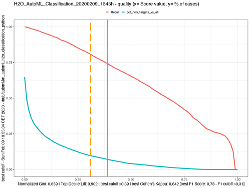
Find the best cut-off point for your model
Gives you the idea where the best cutoff might be by consulting two measures
-
>0.39 score if you follow Cohen’s Kappa -
>0.31 if you follow the best F1 score
There is always a price to pay. The blue curve gives you the % of non-targets with regards to all cases that you would have to carry with you if you choose this specific cutoff
If you choose >0.39 you will capture 74% of all your targets. You will have to ‘carry’ 7% off all your cases that are non-Targets which overall make 67% of your population.
If you choose a cutoff of >0.68 you get nearly 50% of your Targets with only about 2% of the population as non-Targets. If this is good or bad for your business case you would have to decide. For more details see the Excel file.
The accompanying Excel file also holds some interesting information
The Leaderboard from the set of models run
It gives you an idea
- Which types of models were considered?
- Also, the stretch of the AUC could be quite wide. Since all the models only trained 2.5 minutes it would be possible that further training time might result in better models
- In between there as some other models besides GBM if they would appear more often you might also investigate that further
If you are into tweaking, you models further the model summary also gives you the parameters used.
Further information will be stored in the print of the whole model with all parameters, also about the cross-validations done.
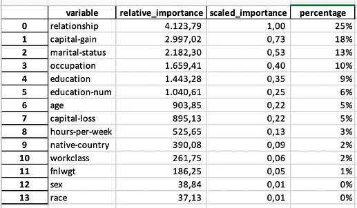
Variable Importance is very important
Then there is the variable importance list. You should study that list carefully. If one variable captures all the importance you might have a leak. And the variables also should make sense.
If you have a very large list and further down, they stop making sense you could cut them off (besides all the data preparation magic you could do with vtreat, featuretools, tsfresh, label encoding and so on). And also, H2O does some modifications.
You could use that list to shrink your y variables and re-run the model. The list of variables is also stored in the overall list.
Fun fact in this case: your relationship and marital status are more important to determine whether you will earn more than $50,000 then your education …
Get an overview how your model is doing in Bins and numbers
I like this sort of table since it gives you an idea about what a cut-off at a certain score (“submission”) would mean.
All numbers are taken from the test/validation group (30% of your population in this case) – you might have to think about your overall population to get the exact proportion.
If you choose a cutoff at 0.8 you would get 92% precision and 43% of all your desired targets. In marketing/cross-selling that would be an excellent result. In credit scoring, you might not want to live with 8% of people not paying back their loans. So again, the cut-off and value of your model very much depends on your business question.
A word about cross-validation
Another aspect of your model quality and stability could be judged by looking at a cross-validation. Although H2O, for example, does a lot of that by default in order to avoid overfitting you might want to do some checks of your own.
The basic idea is: if your model is really catching a general trend and has good rules they should work on all (random) sub-populations and you would expect the model to be quite stable.
Several tests are run. In the end, we look at a combined standard deviation. 0 would represent a perfect match between all subgroups (sub-sampling and leaving one out techniques). So if you would have to choose between several excellent models you might want to consider the one with the least deviation.
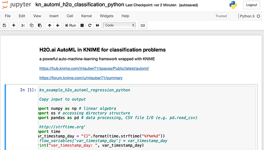
Jupyter notebook
Enclosed in the workflow in the subfolder
/script/ kn_automl_h2o_classification_python.ipynb
there is a walkthrough of Automl in a Jupyter notebook to explore the functions further and if you do not wish to use the wrapper with KNIME



 I’ve let it run about 30mins with the default data you have set and get an AUC of 0.9283 (best model is a GBM). If I train an H2O GBM myself within KNIME using 250 trees and a depth of 6 (training time just a few seconds), I get 0.9292, so I am wondering why the autoML result is worse. I can see that the best model you have trained achieves a better score, 0.9293! Did you use a different configuration for H2O AutoML or simply let it run longer? I can see that you changed the early stopping parameters, those may be interesting to tune. Maybe it’s also just the seed
